Losses

Loss functions for model evaluation.

The most important train signal is the forecast error, which is the difference between the observed value $y_{\tau}$ and the prediction $\hat{y}_{\tau}$, at time $y_{\tau}$:

$$e_{\tau} = y_{\tau}-\hat{y}_{\tau} \qquad \qquad \tau \in \{t+1,\dots,t+H \}$$

The train loss summarizes the forecast errors in different evaluation metrics.

1. Scale-dependent Errors

Mean Absolute Error

$$\mathrm{MAE}(\mathbf{y}_{\tau}, \mathbf{\hat{y}}_{\tau}) = \frac{1}{H} \sum^{t+H}_{\tau=t+1} |y_{\tau} - \hat{y}_{\tau}|$$

mae

mae(df, models, id_col='unique_id', target_col='y', cutoff_col='cutoff')

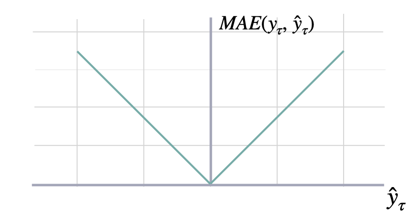
Mean Absolute Error (MAE)

MAE measures the relative prediction accuracy of a forecasting method by calculating the deviation of the prediction and the true value at a given time and averages these devations over the length of the series.

Mean Squared Error

$$\mathrm{MSE}(\mathbf{y}_{\tau}, \mathbf{\hat{y}}_{\tau}) = \frac{1}{H} \sum^{t+H}_{\tau=t+1} (y_{\tau} - \hat{y}_{\tau})^{2}$$

mse

mse(df, models, id_col='unique_id', target_col='y', cutoff_col='cutoff')

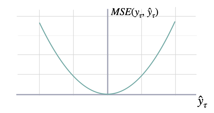
Mean Squared Error (MSE)

MSE measures the relative prediction accuracy of a forecasting method by calculating the squared deviation of the prediction and the true value at a given time, and averages these devations over the length of the series.

Root Mean Squared Error

$$\mathrm{RMSE}(\mathbf{y}_{\tau}, \mathbf{\hat{y}}_{\tau}) = \sqrt{\frac{1}{H} \sum^{t+H}_{\tau=t+1} (y_{\tau} - \hat{y}_{\tau})^{2}}$$

rmse

rmse(df, models, id_col='unique_id', target_col='y', cutoff_col='cutoff')

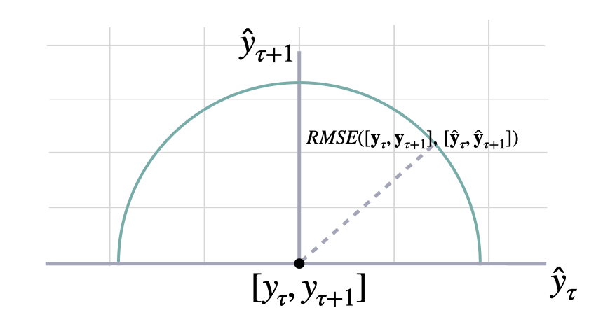
Root Mean Squared Error (RMSE)

RMSE measures the relative prediction accuracy of a forecasting method by calculating the squared deviation of the prediction and the observed value at a given time and averages these devations over the length of the series. Finally the RMSE will be in the same scale as the original time series so its comparison with other series is possible only if they share a common scale. RMSE has a direct connection to the L2 norm.

Bias

$$\mathrm{Bias}(\mathbf{y}_{\tau}, \mathbf{\hat{y}}_{\tau}) = \frac{1}{H} \sum^{t+H}_{\tau=t+1} (\hat{y}_{\tau} - \mathbf{y}_{\tau})$$

bias

bias(df, models, id_col='unique_id', target_col='y', cutoff_col='cutoff')

Forecast estimator bias.

Defined as prediction - actual

Cumulative Forecast Error

$$\mathrm{CFE}(\mathbf{y}_{\tau}, \mathbf{\hat{y}}_{\tau}) = \sum^{t+H}_{\tau=t+1} (\hat{y}_{\tau} - \mathbf{y}_{\tau})$$

cfe

cfe(df, models, id_col='unique_id', target_col='y', cutoff_col='cutoff')

Cumulative Forecast Error (CFE)

Total signed forecast error per series. Positive values mean under forecast; negative mean over forecast.

Absolute Periods In Stock

$$\mathrm{PIS}(\mathbf{y}_{\tau}, \mathbf{\hat{y}}_{\tau}) = \sum^{t+H}_{\tau=t+1} |y_{\tau} - \hat{y}_{\tau}|$$

pis

pis(df, models, id_col='unique_id', target_col='y', cutoff_col='cutoff')

Compute the raw Absolute Periods In Stock (PIS) for one or multiple models.

The PIS metric sums the absolute forecast errors per series without any scaling, yielding a scale-dependent measure of bias.

Linex

$$\mathrm{Linex}(\mathbf{y}_{\tau}, \mathbf{\hat{y}}_{\tau}) = \frac{1}{H} \sum^{t+H}_{\tau=t+1} (e^{a(y_{\tau} - \hat{y}_{\tau})} - a(y_{\tau} - \hat{y}_{\tau}) - 1)$$

where must be $a\neq0$.

linex

linex(df, models, id_col='unique_id', target_col='y', cutoff_col='cutoff', a=1.0)

Linex Loss (Linear Exponential)

The Linex loss penalizes over- and under-forecasting asymmetrically depending on the parameter a.

• If a > 0, under-forecasting ($y > \hat{y}$) is penalized more.
• If a < 0, over-forecasting ($\hat{y} > y$) is penalized more.
• a must not be 0.

Parameters:

Name	Type	Description	Default
a	float	Asymmetry parameter. Must be non-zero. Defaults to 1.0.	1.0

2. Percentage Errors

Mean Absolute Percentage Error

$$\mathrm{MAPE}(\mathbf{y}_{\tau}, \mathbf{\hat{y}}_{\tau}) = \frac{1}{H} \sum^{t+H}_{\tau=t+1} \frac{|y_{\tau}-\hat{y}_{\tau}|}{|y_{\tau}|}$$

mape

mape(df, models, id_col='unique_id', target_col='y', cutoff_col='cutoff')

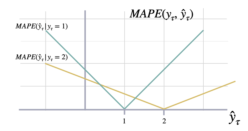
Mean Absolute Percentage Error (MAPE)

MAPE measures the relative prediction accuracy of a forecasting method by calculating the percentual deviation of the prediction and the observed value at a given time and averages these devations over the length of the series. The closer to zero an observed value is, the higher penalty MAPE loss assigns to the corresponding error.

Symmetric Mean Absolute Percentage Error

$$\mathrm{SMAPE}_{2}(\mathbf{y}_{\tau}, \mathbf{\hat{y}}_{\tau}) = \frac{1}{H} \sum^{t+H}_{\tau=t+1} \frac{|y_{\tau}-\hat{y}_{\tau}|}{|y_{\tau}|+|\hat{y}_{\tau}|}$$

smape

smape(df, models, id_col='unique_id', target_col='y', cutoff_col='cutoff')

Symmetric Mean Absolute Percentage Error (SMAPE)

SMAPE measures the relative prediction accuracy of a forecasting method by calculating the relative deviation of the prediction and the observed value scaled by the sum of the absolute values for the prediction and observed value at a given time, then averages these devations over the length of the series. This allows the SMAPE to have bounds between 0% and 100% which is desirable compared to normal MAPE that may be undetermined when the target is zero.

3. Scale-independent Errors

Mean Absolute Scaled Error

$$\mathrm{MASE}(\mathbf{y}_{\tau}, \mathbf{\hat{y}}_{\tau}, \mathbf{\hat{y}}^{season}_{\tau}) = \frac{1}{H} \sum^{t+H}_{\tau=t+1} \frac{|y_{\tau}-\hat{y}_{\tau}|}{\mathrm{MAE}(\mathbf{y}_{\tau}, \mathbf{\hat{y}}^{season}_{\tau})}$$

mase

mase(df, models, seasonality, train_df, id_col='unique_id', target_col='y', cutoff_col='cutoff', time_col='ds')

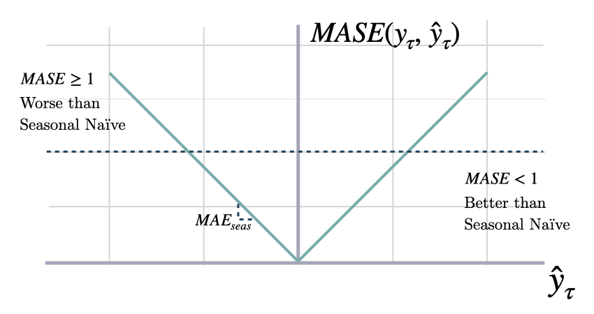
Mean Absolute Scaled Error (MASE)

MASE measures the relative prediction accuracy of a forecasting method by comparinng the mean absolute errors of the prediction and the observed value against the mean absolute errors of the seasonal naive model. The MASE partially composed the Overall Weighted Average (OWA), used in the M4 Competition.

Parameters:

Name	Type	Description	Default
df	pandas or polars DataFrame	Input dataframe with id, actuals and predictions.	required
models	list of str	Columns that identify the models predictions.	required
seasonality	int	Main frequency of the time series; Hourly 24, Daily 7, Weekly 52, Monthly 12, Quarterly 4, Yearly 1.	required
train_df	pandas or polars DataFrame	Training dataframe with id and actual values. Must be sorted by time.	required
id_col	str	Column that identifies each serie. Defaults to ‘unique_id’.	‘unique_id’
target_col	str	Column that contains the target. Defaults to ‘y’.	‘y’
cutoff_col	str	Column that identifies the cutoff point for each forecast cross-validation fold. Defaults to ‘cutoff’.	‘cutoff’

Returns:

Type	Description
IntoDataFrameT	pandas or polars DataFrame: dataframe with one row per id and one column per model.

Relative Mean Absolute Error

$$\mathrm{RMAE}(\mathbf{y}_{\tau}, \mathbf{\hat{y}}_{\tau}, \mathbf{\hat{y}}^{base}_{\tau}) = \frac{1}{H} \sum^{t+H}_{\tau=t+1} \frac{|y_{\tau}-\hat{y}_{\tau}|}{\mathrm{MAE}(\mathbf{y}_{\tau}, \mathbf{\hat{y}}^{base}_{\tau})}$$

rmae

rmae(df, models, baseline, id_col='unique_id', target_col='y', cutoff_col='cutoff')

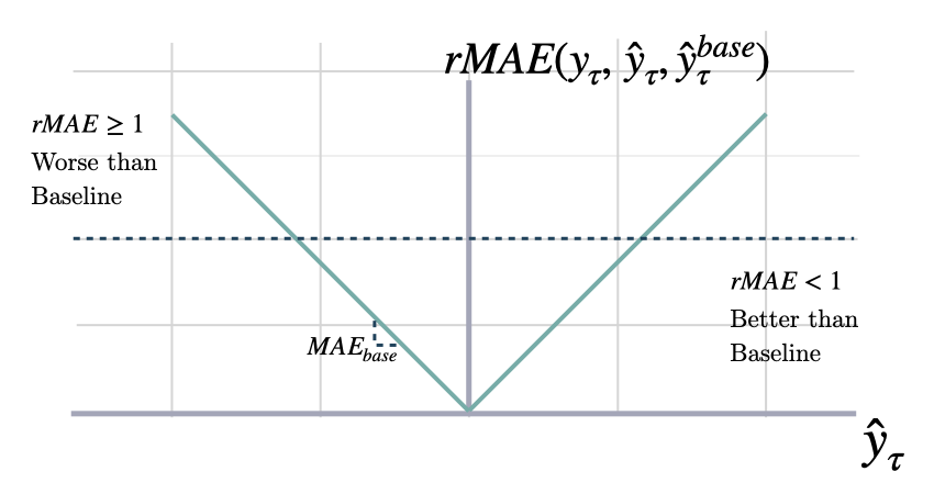
Relative Mean Absolute Error (RMAE)

Calculates the RAME between two sets of forecasts (from two different forecasting methods). A number smaller than one implies that the forecast in the numerator is better than the forecast in the denominator.

Parameters:

Name	Type	Description	Default
df	pandas or polars DataFrame	Input dataframe with id, times, actuals and predictions.	required
models	list of str	Columns that identify the models predictions.	required
baseline	str	Column that identifies the baseline model predictions.	required
id_col	str	Column that identifies each serie. Defaults to ‘unique_id’.	‘unique_id’
target_col	str	Column that contains the target. Defaults to ‘y’.	‘y’
cutoff_col	str	Column that identifies the cutoff point for each forecast cross-validation fold. Defaults to ‘cutoff’.	‘cutoff’

Returns:

Type	Description
IntoDataFrameT	pandas or polars DataFrame: dataframe with one row per id and one column per model.

Normalized Deviation

$$\mathrm{ND}(\mathbf{y}_{\tau}, \mathbf{\hat{y}}_{\tau}) = \frac{\sum^{t+H}_{\tau=t+1} |y_{\tau} - \hat{y}_{\tau}|}{\sum^{t+H}_{\tau=t+1} | y_{\tau} |}$$

nd

nd(df, models, id_col='unique_id', target_col='y', cutoff_col='cutoff')

Normalized Deviation (ND)

ND measures the relative prediction accuracy of a forecasting method by calculating the sum of the absolute deviation of the prediction and the true value at a given time and dividing it by the sum of the absolute value of the ground truth.

Mean Squared Scaled Error

$$\mathrm{MSSE}(\mathbf{y}_{\tau}, \mathbf{\hat{y}}_{\tau}, \mathbf{\hat{y}}^{season}_{\tau}) = \frac{1}{H} \sum^{t+H}_{\tau=t+1} \frac{(y_{\tau}-\hat{y}_{\tau})^2}{\mathrm{MSE}(\mathbf{y}_{\tau}, \mathbf{\hat{y}}^{season}_{\tau})}$$

msse

msse(df, models, seasonality, train_df, id_col='unique_id', target_col='y', cutoff_col='cutoff', time_col='ds')

Mean Squared Scaled Error (MSSE)

MSSE measures the relative prediction accuracy of a forecasting method by comparinng the mean squared errors of the prediction and the observed value against the mean squared errors of the seasonal naive model.

Parameters:

Name	Type	Description	Default
df	pandas or polars DataFrame	Input dataframe with id, actuals and predictions.	required
models	list of str	Columns that identify the models predictions.	required
seasonality	int	Main frequency of the time series; Hourly 24, Daily 7, Weekly 52, Monthly 12, Quarterly 4, Yearly 1.	required
train_df	pandas or polars DataFrame	Training dataframe with id and actual values. Must be sorted by time.	required
id_col	str	Column that identifies each serie. Defaults to ‘unique_id’.	‘unique_id’
target_col	str	Column that contains the target. Defaults to ‘y’.	‘y’
cutoff_col	str	Column that identifies the cutoff point for each forecast cross-validation fold. Defaults to ‘cutoff’.	‘cutoff’

Returns:

Type	Description
IntoDataFrameT	pandas or polars DataFrame: dataframe with one row per id and one column per model.

Root Mean Squared Scaled Error

$$\mathrm{RMSSE}(\mathbf{y}_{\tau}, \mathbf{\hat{y}}_{\tau}, \mathbf{\hat{y}}^{season}_{\tau}) = \sqrt{\frac{1}{H} \sum^{t+H}_{\tau=t+1} \frac{(y_{\tau}-\hat{y}_{\tau})^2}{\mathrm{MSE}(\mathbf{y}_{\tau}, \mathbf{\hat{y}}^{season}_{\tau})}}$$

rmsse

rmsse(df, models, seasonality, train_df, id_col='unique_id', target_col='y', cutoff_col='cutoff', time_col='ds')

Root Mean Squared Scaled Error (RMSSE)

MSSE measures the relative prediction accuracy of a forecasting method by comparinng the mean squared errors of the prediction and the observed value against the mean squared errors of the seasonal naive model.

Parameters:

Name	Type	Description	Default
df	pandas or polars DataFrame	Input dataframe with id, actuals and predictions.	required
models	list of str	Columns that identify the models predictions.	required
seasonality	int	Main frequency of the time series; Hourly 24, Daily 7, Weekly 52, Monthly 12, Quarterly 4, Yearly 1.	required
train_df	pandas or polars DataFrame	Training dataframe with id and actual values. Must be sorted by time.	required
id_col	str	Column that identifies each serie. Defaults to ‘unique_id’.	required
target_col	str	Column that contains the target. Defaults to ‘y’.	required
cutoff_col	str	Column that identifies the cutoff point for each forecast cross-validation fold. Defaults to ‘cutoff’.	required

Returns:

Type	Description
pandas or polars DataFrame: dataframe with one row per id and one column per model.

Scaled Absolute Periods In Stock

$$\mathrm{PIS}(\mathbf{y}_{\tau}, \mathbf{\hat{y}}_{\tau}) = \sum^{t+H}_{\tau=t+1} \frac{|y_{\tau} - \hat{y}_{\tau}|}{\bar{y}}$$

where $\bar{y}=\frac{1}{H}\sum^{t+H}_{\tau=t+1} y_{\tau}$.

spis

spis(df, models, train_df, id_col='unique_id', target_col='y', cutoff_col='cutoff', time_col='ds')

Compute the scaled Absolute Periods In Stock (sAPIS) for one or multiple models.

The sPIS metric scales the sum of absolute forecast errors by the mean in-sample demand, yielding a scale-independent bias measure that can be aggregated across series.

Parameters:

Name	Type	Description	Default
df	pandas or polars DataFrame	Input dataframe with id, actuals and predictions.	required
models	list of str	Columns that identify the models predictions.	required
train_df	pandas or polars DataFrame	Training dataframe with id and actual values. Must be sorted by time.	required
id_col	str	Column that identifies each serie. Defaults to ‘unique_id’.	‘unique_id’
target_col	str	Column that contains the target. Defaults to ‘y’.	‘y’
cutoff_col	str	Column that identifies the cutoff point for each forecast cross-validation fold. Defaults to ‘cutoff’.	‘cutoff’

Returns:

Type	Description
IntoDataFrameT	pandas or polars DataFrame: dataframe with one row per id and one column per model.

4. Probabilistic Errors

Quantile Loss

$$\mathrm{QL}(\mathbf{y}_{\tau}, \mathbf{\hat{y}}^{(q)}_{\tau}) = \frac{1}{H} \sum^{t+H}_{\tau=t+1} \Big( (1-q)\,( \hat{y}^{(q)}_{\tau} - y_{\tau} )_{+} + q\,( y_{\tau} - \hat{y}^{(q)}_{\tau} )_{+} \Big)$$

quantile_loss

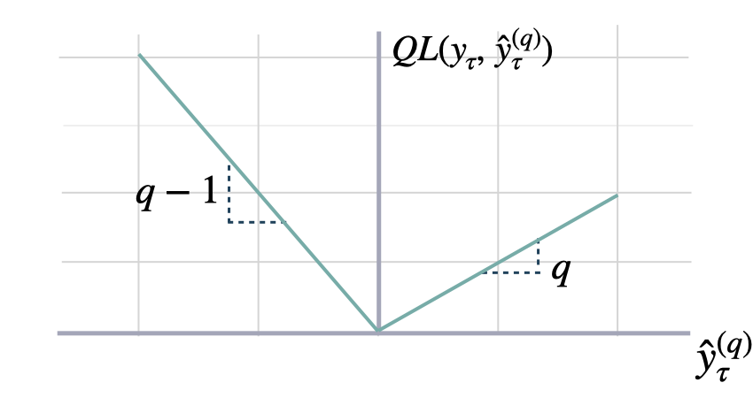
quantile_loss(df, models, q=0.5, id_col='unique_id', target_col='y', cutoff_col='cutoff')

Quantile Loss (QL)

QL measures the deviation of a quantile forecast. By weighting the absolute deviation in a non symmetric way, the loss pays more attention to under or over estimation. A common value for q is 0.5 for the deviation from the median.

Parameters:

Name	Type	Description	Default
df	pandas or polars DataFrame	Input dataframe with id, times, actuals and predictions.	required
models	dict from str to str	Mapping from model name to the model predictions for the specified quantile.	required
q	float	Quantile for the predictions’ comparison. Defaults to 0.5.	0.5
id_col	str	Column that identifies each serie. Defaults to ‘unique_id’.	‘unique_id’
target_col	str	Column that contains the target. Defaults to ‘y’.	‘y’
cutoff_col	str	Column that identifies the cutoff point for each forecast cross-validation fold. Defaults to ‘cutoff’.	‘cutoff’

Returns:

Type	Description
IntoDataFrameT	pandas or polars DataFrame: dataframe with one row per id and one column per model.

Scaled Quantile Loss

$$\mathrm{SQL}(\mathbf{y}_{\tau}, \mathbf{\hat{y}}^{(q)}_{\tau}) = \frac{1}{H} \sum^{t+H}_{\tau=t+1} \frac{(1-q)\,( \hat{y}^{(q)}_{\tau} - y_{\tau} )_{+} + q\,( y_{\tau} - \hat{y}^{(q)}_{\tau} )_{+}}{\mathrm{MAE}(\mathbf{y}_{\tau}, \mathbf{\hat{y}}^{season}_{\tau})}$$

scaled_quantile_loss

scaled_quantile_loss(df, models, seasonality, train_df, q=0.5, id_col='unique_id', target_col='y', cutoff_col='cutoff', time_col='ds')

Scaled Quantile Loss (SQL)

SQL measures the deviation of a quantile forecast scaled by the mean absolute errors of the seasonal naive model. By weighting the absolute deviation in a non symmetric way, the loss pays more attention to under or over estimation. A common value for q is 0.5 for the deviation from the median. This was the official measure used in the M5 Uncertainty competition with seasonality = 1.

Parameters:

Name	Type	Description	Default
df	pandas or polars DataFrame	Input dataframe with id, times, actuals and predictions.	required
models	dict from str to str	Mapping from model name to the model predictions for the specified quantile.	required
seasonality	int	Main frequency of the time series; Hourly 24, Daily 7, Weekly 52, Monthly 12, Quarterly 4, Yearly 1.	required
train_df	pandas or polars DataFrame	Training dataframe with id and actual values. Must be sorted by time.	required
q	float	Quantile for the predictions’ comparison. Defaults to 0.5.	0.5
id_col	str	Column that identifies each serie. Defaults to ‘unique_id’.	‘unique_id’
target_col	str	Column that contains the target. Defaults to ‘y’.	‘y’
cutoff_col	str	Column that identifies the cutoff point for each forecast cross-validation fold. Defaults to ‘cutoff’.	‘cutoff’

Returns:

Type	Description
IntoDataFrameT	pandas or polars DataFrame: dataframe with one row per id and one column per model.

Multi-Quantile Loss

$$\mathrm{MQL}(\mathbf{y}_{\tau}, [\mathbf{\hat{y}}^{(q_{1})}_{\tau}, ... ,\hat{y}^{(q_{n})}_{\tau}]) = \frac{1}{n} \sum_{q_{i}} \mathrm{QL}(\mathbf{y}_{\tau}, \mathbf{\hat{y}}^{(q_{i})}_{\tau})$$

mqloss

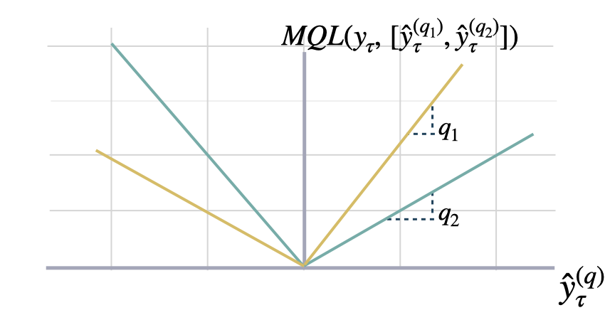
mqloss(df, models, quantiles, id_col='unique_id', target_col='y', cutoff_col='cutoff')

Multi-Quantile loss (MQL)

MQL calculates the average multi-quantile Loss for a given set of quantiles, based on the absolute difference between predicted quantiles and observed values.

The limit behavior of MQL allows to measure the accuracy of a full predictive distribution with the continuous ranked probability score (CRPS). This can be achieved through a numerical integration technique, that discretizes the quantiles and treats the CRPS integral with a left Riemann approximation, averaging over uniformly distanced quantiles.

Parameters:

Name	Type	Description	Default
df	pandas or polars DataFrame	Input dataframe with id, times, actuals and predictions.	required
models	dict from str to list of str	Mapping from model name to the model predictions for each quantile.	required
quantiles	numpy array	Quantiles to compare against.	required
id_col	str	Column that identifies each serie. Defaults to ‘unique_id’.	‘unique_id’
target_col	str	Column that contains the target. Defaults to ‘y’.	‘y’
cutoff_col	str	Column that identifies the cutoff point for each forecast cross-validation fold. Defaults to ‘cutoff’.	‘cutoff’

Returns:

Type	Description
IntoDataFrameT	pandas or polars DataFrame: dataframe with one row per id and one column per model.

Scaled Multi-Quantile Loss

$$\mathrm{MQL}(\mathbf{y}_{\tau}, [\mathbf{\hat{y}}^{(q_{1})}_{\tau}, ... ,\hat{y}^{(q_{n})}_{\tau}]) = \frac{1}{n} \sum_{q_{i}} \frac{\mathrm{QL}(\mathbf{y}_{\tau}, \mathbf{\hat{y}}^{(q_{i})}_{\tau})}{\mathrm{MAE}(\mathbf{y}_{\tau}, \mathbf{\hat{y}}^{season}_{\tau})}$$

scaled_mqloss

scaled_mqloss(df, models, quantiles, seasonality, train_df, id_col='unique_id', target_col='y', cutoff_col='cutoff', time_col='ds')

Scaled Multi-Quantile loss (SMQL)

SMQL calculates the average multi-quantile Loss for a given set of quantiles, based on the absolute difference between predicted quantiles and observed values scaled by the mean absolute errors of the seasonal naive model. The limit behavior of MQL allows to measure the accuracy of a full predictive distribution with the continuous ranked probability score (CRPS). This can be achieved through a numerical integration technique, that discretizes the quantiles and treats the CRPS integral with a left Riemann approximation, averaging over uniformly distanced quantiles. This was the official measure used in the M5 Uncertainty competition with seasonality = 1.

Parameters:

Name	Type	Description	Default
df	pandas or polars DataFrame	Input dataframe with id, times, actuals and predictions.	required
models	dict from str to list of str	Mapping from model name to the model predictions for each quantile.	required
quantiles	numpy array	Quantiles to compare against.	required
seasonality	int	Main frequency of the time series; Hourly 24, Daily 7, Weekly 52, Monthly 12, Quarterly 4, Yearly 1.	required
train_df	pandas or polars DataFrame	Training dataframe with id and actual values. Must be sorted by time.	required
id_col	str	Column that identifies each serie. Defaults to ‘unique_id’.	‘unique_id’
target_col	str	Column that contains the target. Defaults to ‘y’.	‘y’
cutoff_col	str	Column that identifies the cutoff point for each forecast cross-validation fold. Defaults to ‘cutoff’.	‘cutoff’

Returns:

Type	Description
IntoDataFrameT	pandas or polars DataFrame: dataframe with one row per id and one column per model.

Coverage

coverage

coverage(df, models, level, id_col='unique_id', target_col='y', cutoff_col='cutoff')

Coverage of y with y_hat_lo and y_hat_hi.

Parameters:

Name	Type	Description	Default
df	pandas or polars DataFrame	Input dataframe with id, times, actuals and predictions.	required
models	list of str	Columns that identify the models predictions.	required
level	int	Confidence level used for intervals.	required
id_col	str	Column that identifies each serie. Defaults to ‘unique_id’.	‘unique_id’
target_col	str	Column that contains the target. Defaults to ‘y’.	‘y’
cutoff_col	str	Column that identifies the cutoff point for each forecast cross-validation fold. Defaults to ‘cutoff’.	‘cutoff’

Returns:

Type	Description
IntoDataFrameT	pandas or polars DataFrame: dataframe with one row per id and one column per model.

Calibration

calibration

calibration(df, models, id_col='unique_id', target_col='y', cutoff_col='cutoff')

Fraction of y that is lower than the model’s predictions.

Parameters:

Name	Type	Description	Default
df	pandas or polars DataFrame	Input dataframe with id, times, actuals and predictions.	required
models	dict from str to str	Mapping from model name to the model predictions.	required
id_col	str	Column that identifies each serie. Defaults to ‘unique_id’.	‘unique_id’
target_col	str	Column that contains the target. Defaults to ‘y’.	‘y’
cutoff_col	str	Column that identifies the cutoff point for each forecast cross-validation fold. Defaults to ‘cutoff’.	‘cutoff’

Returns:

Type	Description
IntoDataFrameT	pandas or polars DataFrame: dataframe with one row per id and one column per model.

CRPS

$$\mathrm{sCRPS}(\hat{F}_{\tau}, \mathbf{y}_{\tau}) = \frac{2}{N} \sum_{i} \int^{1}_{0} \frac{\mathrm{QL}(\hat{F}_{i,\tau}, y_{i,\tau})_{q}}{\sum_{i} | y_{i,\tau} |} dq$$

Where $\hat{F}_{\tau}$ is the an estimated multivariate distribution, and $y_{i,\tau}$ are its realizations.

scaled_crps

scaled_crps(df, models, quantiles, id_col='unique_id', target_col='y', cutoff_col='cutoff')

Scaled Continues Ranked Probability Score

Calculates a scaled variation of the CRPS, as proposed by Rangapuram (2021), to measure the accuracy of predicted quantiles y_hat compared to the observation y. This metric averages percentual weighted absolute deviations as defined by the quantile losses.

Parameters:

Name	Type	Description	Default
df	pandas or polars DataFrame	Input dataframe with id, times, actuals and predictions.	required
models	dict from str to list of str	Mapping from model name to the model predictions for each quantile.	required
quantiles	numpy array	Quantiles to compare against.	required
id_col	str	Column that identifies each serie. Defaults to ‘unique_id’.	‘unique_id’
target_col	str	Column that contains the target. Defaults to ‘y’.	‘y’
cutoff_col	str	Column that identifies the cutoff point for each forecast cross-validation fold. Defaults to ‘cutoff’.	‘cutoff’

Returns:

Type	Description
IntoDataFrameT	pandas or polars DataFrame: dataframe with one row per id and one column per model.

Tweedie Deviance

For a set of forecasts $\{\mu_i\}_{i=1}^N$ and observations $\{y_i\}_{i=1}^N$, the mean Tweedie deviance with power $p$ is

$$\mathrm{TD}_{p}(\boldsymbol{\mu}, \mathbf{y}) = \frac{1}{N} \sum_{i=1}^{N} d_{p}(y_i, \mu_i)$$

where the unit-scaled deviance for each pair $(y,\mu)$ is

$$d_{p}(y,\mu) = 2 \begin{cases} \displaystyle \frac{y^{2-p}}{(1-p)(2-p)} \;-\; \frac{y\,\mu^{1-p}}{1-p} \;+\; \frac{\mu^{2-p}}{2-p}, & p \notin\{1,2\},\\[1em] \displaystyle y\,\ln\!\frac{y}{\mu}\;-\;(y-\mu), & p = 1\quad(\text{Poisson deviance}),\\[0.5em] \displaystyle -2\Bigl[\ln\!\frac{y}{\mu}\;-\;\frac{y-\mu}{\mu}\Bigr], & p = 2\quad(\text{Gamma deviance}). \end{cases}$$

• $y_i$ are the true values, $\mu_i$ the predicted means.
• $p$ controls the variance relationship $\mathrm{Var}(Y)\propto\mu^{p}$.
• When $1<p<2$, this smoothly interpolates between Poisson ($p=1$) and Gamma ($p=2$) deviance.

tweedie_deviance

tweedie_deviance(df, models, power=1.5, id_col='unique_id', target_col='y', cutoff_col='cutoff')

Compute the Tweedie deviance loss for one or multiple models, grouped by an identifier.

Each group’s deviance is calculated using the mean_tweedie_deviance function, which measures the deviation between actual and predicted values under the Tweedie distribution.

The power parameter defines the specific compound distribution:

• 1: Poisson
• (1, 2): Compound Poisson-Gamma
• 2: Gamma

• 2: Inverse Gaussian

Parameters:

Name	Type	Description	Default
df	pandas or polars DataFrame	Input dataframe with id, actuals and predictions.	required
models	list of str	Columns that identify the models predictions.	required
power	float	Tweedie power parameter. Determines the compound distribution. Defaults to 1.5.	1.5
id_col	str	Column that identifies each serie. Defaults to ‘unique_id’.	‘unique_id’
target_col	str	Column that contains the target. Defaults to ‘y’.	‘y’
cutoff_col	str	Column that identifies the cutoff point for each forecast cross-validation fold. Defaults to ‘cutoff’.	‘cutoff’

Returns:

Type	Description
IntoDataFrameT	pandas or polars DataFrame: DataFrame with one row per id and one column per model, containing the mean Tweedie deviance.