

Generate correlated sample paths for scenario analysis
Simulation vs. Prediction Intervals: When to Use Which
NeuralForecast provides two complementary approaches for reasoning about future uncertainty:Prediction Intervals (predict(level=...))
Prediction intervals answer: “What range of values is the target
likely to fall within at each future time step?”
- Output: Independent confidence bands per horizon step (e.g., 90% interval at step ).
- Each step is treated marginally — no information about how steps relate to each other.
- Best for: monitoring, alerting, dashboarding, reporting confidence bands.
Simulation Paths (simulate(...))
Simulation paths answer: “What are realistic joint future
trajectories the time series could follow?”
- Output: complete trajectories of length , each representing a plausible future.
- Temporal correlations between steps are preserved — if step is high, step is likely high too.
- Best for: scenario analysis, portfolio optimization, supply chain planning, energy dispatch, risk assessment (VaR/CVaR), stochastic programming.
Key Difference: Marginal vs. Joint
Consider electricity price forecasting over 24 hours. A 90% prediction interval tells you the price at hour 12 will likely be between $40 and $80. But it says nothing about whether hours 11, 12, and 13 will all be high simultaneously (a sustained price spike) or whether high and low values alternate randomly. Simulation paths capture this joint structure. From 500 simulated paths you can compute: - P(total cost > budget) — requires summing across correlated hours - P(at least 3 consecutive hours above $70) — requires temporal ordering - Expected shortfall (CVaR) — requires the joint tail distribution These questions cannot be answered from marginal prediction intervals alone.Available Simulation Methods
Compatible losses: -
DistributionLoss (Normal, StudentT,
Poisson, etc.) and mixture losses (GMM, PMM, NBMM) — produce
arbitrary quantiles natively. - MQLoss / HuberMQLoss — uses
the model’s trained quantile grid. - IQLoss / HuberIQLoss —
evaluates multiple quantiles via repeated forward passes. - Point
losses (MAE, MSE, etc.) — requires prediction_intervals
(Conformal Prediction) set during fit() to build a quantile grid from
calibration scores.
1. Setup
2. Load Data
We use the AirPassengers dataset — a classic monthly time series of airline passenger counts.3. Train Models
We train five models showcasing different loss types: - NHITS + GMM — Gaussian Mixture Model, a mixtureDistributionLoss. - NHITS +
DistributionLoss(Normal) — parametric distribution output. - NHITS +
MQLoss — Multi-Quantile Loss, directly optimizes quantile levels. -
NHITS + IQLoss — Implicit Quantile Loss, can evaluate any quantile
at inference. - NHITS + MAE with Conformal Prediction — point-loss
model with calibrated prediction intervals.
Since the MAE model needs conformal prediction intervals, we pass
prediction_intervals to fit().
4. Prediction Intervals (Baseline)
First, let’s see the standard prediction intervals — these are marginal (per-step) uncertainty bands.
5. Simulation Paths
Now let’s generate correlated simulation paths using thesimulate()
method. This returns a long-format DataFrame with columns
[unique_id, ds, sample_id, model_1, model_2, ...].
Plotting helper
Generate simulation paths
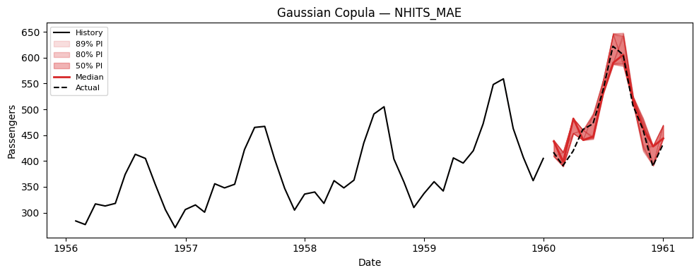
simulate() generates n_paths correlated sample paths for every model
× series combination.
Visualize paths for each model
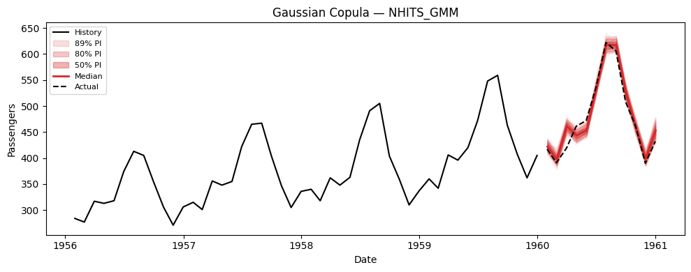
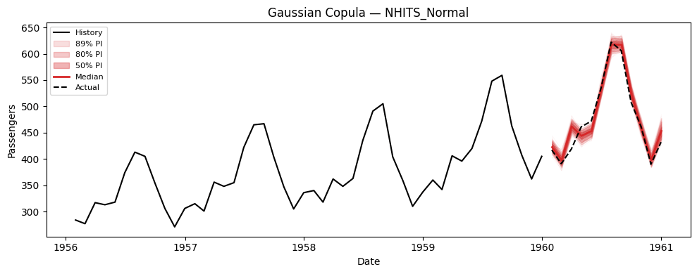
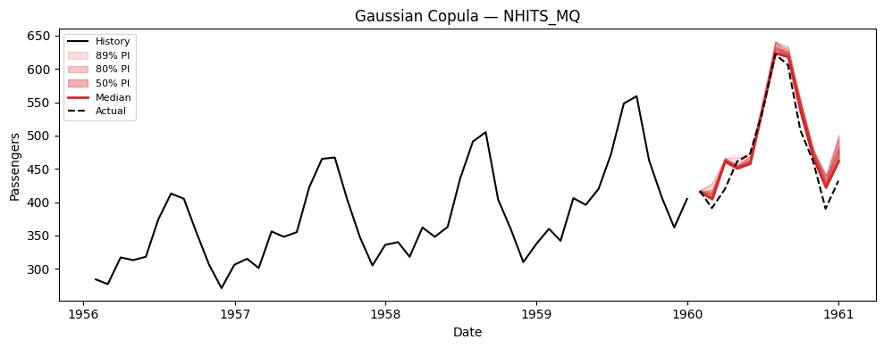
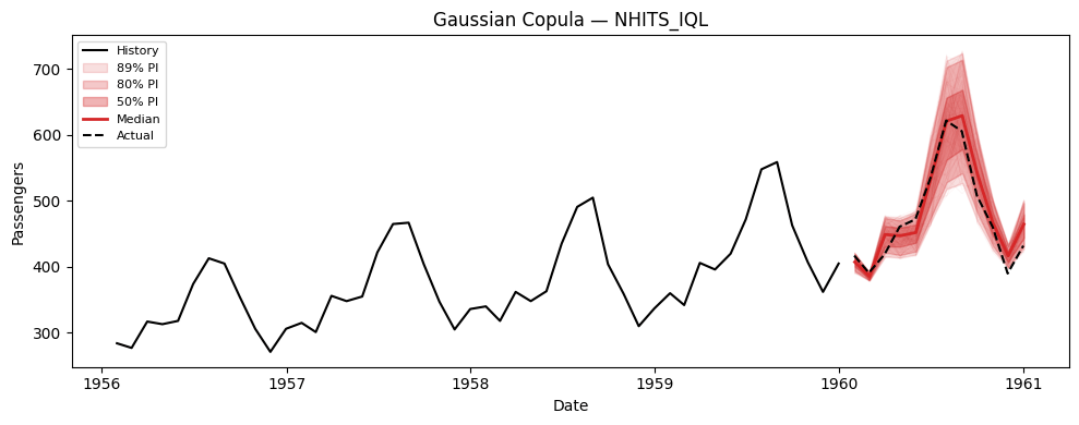
6. Using Simulation Paths for Decision-Making
The key advantage of simulation paths over prediction intervals is answering joint probabilistic questions. Here are concrete examples.Example: Probability of exceeding a cumulative threshold
Suppose we have a capacity of 5,800 total passengers over the next 12 months. What is the probability of exceeding this capacity? This question requires the joint distribution — it cannot be answered from marginal intervals.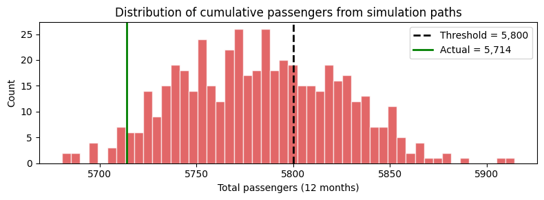
7. Comparing Simulation Methods: Gaussian Copula vs. Schaake Shuffle
Both methods use the same marginal quantile forecasts but differ in how they introduce temporal correlation across horizon steps. Let’s compare them on the NHITS_Normal model.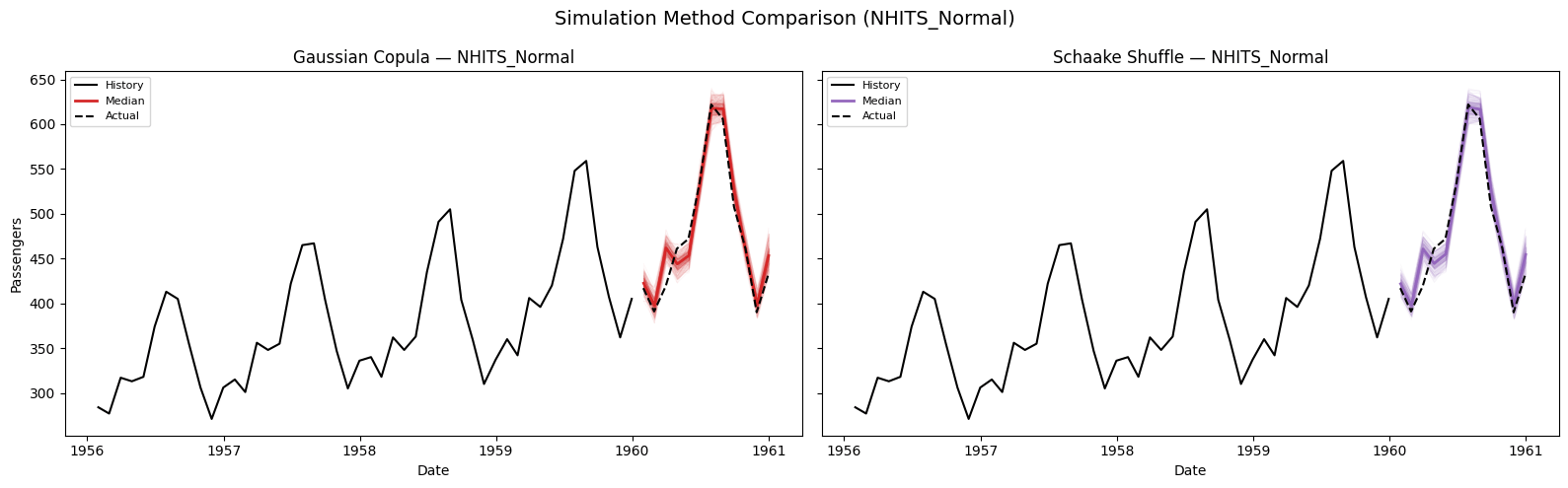
Diagnosing the dependence structure
The path bundles above look nearly identical, and they should: both methods share the same marginal quantiles, so any per-step summary — the median line, the shaded intervals — is by construction the same. The methods differ only in the joint structure, which no marginal view can reveal. Two diagnostics that do reveal it: the step-to-step rank correlation of the paths, and the mean longest run of consecutive months above their own median. Both are compared against the same statistics on the historical rolling windows (the Schaake shuffle’s own templates) and against a null built by permuting each step independently — identical marginals, dependence destroyed.8. Evaluating Marginal vs. Joint Distributions
We can evaluate both the marginal distribution (frompredict(quantiles=...)) and the joint distribution (from
simulate()) using the same metrics. For each model we compare:
- Point metrics: MAE, MSE on the median forecast.
- Probabilistic metric: scaled CRPS on the quantile forecasts —
either from
predict(marginal) or derived from simulation paths (joint).
Interpreting the results:
- MAE / MSE (point metrics): Both simulation methods use the median of the sample paths as their point forecast. Since the marginal quantiles and simulation-derived quantiles share the same underlying model, the median forecasts are similar but not identical — simulation introduces sampling variability.
- Scaled CRPS (probabilistic metric): Measures the quality of the
full quantile distribution. The marginal quantiles come directly
from the model’s predictive distribution, while the
simulation-derived quantiles are empirical (computed from
n_pathssamples). With enough paths, the simulation CRPS should converge to the marginal CRPS.
9. Summary
Simulation Methods
Compatible Losses
References
- Baron, E. et al. (2025). Efficiently generating correlated sample paths from multi-step time series foundation models. NeurIPS 2025 Workshop.
- Clark, M. et al. (2004). The Schaake shuffle: A method for reconstructing space-time variability. Journal of Hydrometeorology, 5(1).