Long-Horizon Forecasting with NHITS

Long-horizon forecasting is challenging because of the volatility of the predictions and the computational complexity. To solve this problem we created the NHITS model and made the code available NeuralForecast library. NHITS specializes its partial outputs in the different frequencies of the time series through hierarchical interpolation and multi-rate input processing.

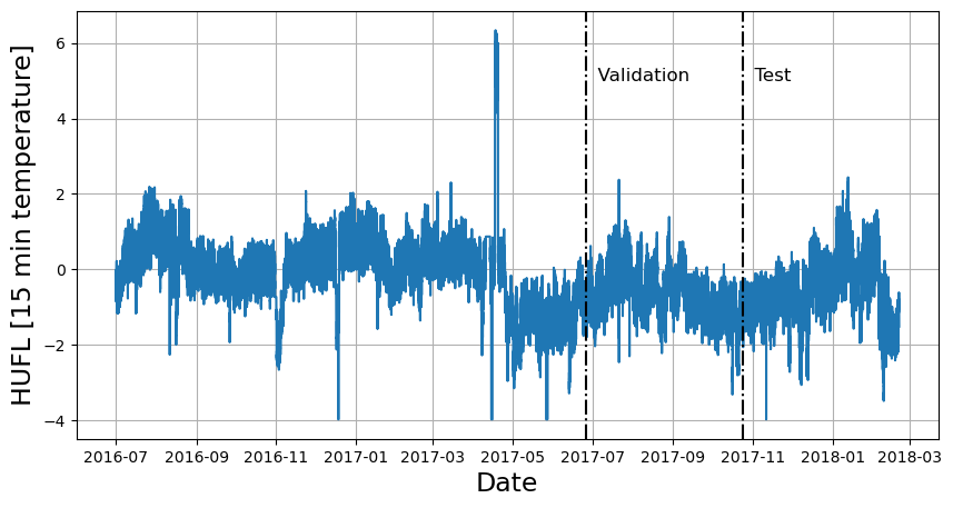
In this notebook we show how to use NHITS on the ETTm2 benchmark dataset. This data set includes data points for 2 Electricity Transformers at 2 stations, including load, oil temperature.

We will show you how to load data, train, and perform automatic hyperparameter tuning, to achieve SoTA performance, outperforming even the latest Transformer architectures for a fraction of their computational cost (50x faster).

You can run these experiments using GPU with Google Colab.

1. Installing NeuralForecast

%%capture
!pip install neuralforecast datasetsforecast utilsforecast

2. Load ETTm2 Data

The LongHorizon class will automatically download the complete ETTm2 dataset and process it.

It return three Dataframes: Y_df contains the values for the target variables, X_df contains exogenous calendar features and S_df contains static features for each time-series (none for ETTm2). For this example we will only use Y_df.

If you want to use your own data just replace Y_df. Be sure to use a long format and have a similar structure to our data set.

import pandas as pd
from datasetsforecast.long_horizon import LongHorizon

# Change this to your own data to try the model
Y_df, _, _ = LongHorizon.load(directory='./', group='ETTm2')
Y_df['ds'] = pd.to_datetime(Y_df['ds'])

# For this excercise we are going to take 20% of the DataSet
n_time = len(Y_df.ds.unique())
val_size = int(.2 * n_time)
test_size = int(.2 * n_time)

Y_df.groupby('unique_id').head(2)

	unique_id	ds	y
0	HUFL	2016-07-01 00:00:00	-0.041413
1	HUFL	2016-07-01 00:15:00	-0.185467
57600	HULL	2016-07-01 00:00:00	0.040104
57601	HULL	2016-07-01 00:15:00	-0.214450
115200	LUFL	2016-07-01 00:00:00	0.695804
115201	LUFL	2016-07-01 00:15:00	0.434685
172800	LULL	2016-07-01 00:00:00	0.434430
172801	LULL	2016-07-01 00:15:00	0.428168
230400	MUFL	2016-07-01 00:00:00	-0.599211
230401	MUFL	2016-07-01 00:15:00	-0.658068
288000	MULL	2016-07-01 00:00:00	-0.393536
288001	MULL	2016-07-01 00:15:00	-0.659338
345600	OT	2016-07-01 00:00:00	1.018032
345601	OT	2016-07-01 00:15:00	0.980124

import matplotlib.pyplot as plt

# We are going to plot the temperature of the transformer 
# and marking the validation and train splits
u_id = 'HUFL'
x_plot = pd.to_datetime(Y_df[Y_df.unique_id==u_id].ds)
y_plot = Y_df[Y_df.unique_id==u_id].y.values

x_val = x_plot[n_time - val_size - test_size]
x_test = x_plot[n_time - test_size]

fig = plt.figure(figsize=(10, 5))
fig.tight_layout()

plt.plot(x_plot, y_plot)
plt.xlabel('Date', fontsize=17)
plt.ylabel('HUFL [15 min temperature]', fontsize=17)

plt.axvline(x_val, color='black', linestyle='-.')
plt.axvline(x_test, color='black', linestyle='-.')
plt.text(x_val, 5, '  Validation', fontsize=12)
plt.text(x_test, 5, '  Test', fontsize=12)

plt.grid()

3. Hyperparameter selection and forecasting

The AutoNHITS class will automatically perform hyperparamter tunning using Tune library, exploring a user-defined or default search space. Models are selected based on the error on a validation set and the best model is then stored and used during inference.

The AutoNHITS.default_config attribute contains a suggested hyperparameter space. Here, we specify a different search space following the paper’s hyperparameters. Notice that 1000 Stochastic Gradient Steps are enough to achieve SoTA performance. Feel free to play around with this space.

from ray import tune
from neuralforecast.auto import AutoNHITS
from neuralforecast.core import NeuralForecast

horizon = 96 # 24hrs = 4 * 15 min.

# Use your own config or AutoNHITS.default_config
nhits_config = {
       "learning_rate": tune.choice([1e-3]),                                     # Initial Learning rate
       "max_steps": tune.choice([1000]),                                         # Number of SGD steps
       "input_size": tune.choice([5 * horizon]),                                 # input_size = multiplier * horizon
       "batch_size": tune.choice([7]),                                           # Number of series in windows
       "windows_batch_size": tune.choice([256]),                                 # Number of windows in batch
       "n_pool_kernel_size": tune.choice([[2, 2, 2], [16, 8, 1]]),               # MaxPool's Kernelsize
       "n_freq_downsample": tune.choice([[168, 24, 1], [24, 12, 1], [1, 1, 1]]), # Interpolation expressivity ratios
       "activation": tune.choice(['ReLU']),                                      # Type of non-linear activation
       "n_blocks":  tune.choice([[1, 1, 1]]),                                    # Blocks per each 3 stacks
       "mlp_units":  tune.choice([[[512, 512], [512, 512], [512, 512]]]),        # 2 512-Layers per block for each stack
       "interpolation_mode": tune.choice(['linear']),                            # Type of multi-step interpolation
       "val_check_steps": tune.choice([100]),                                    # Compute validation every 100 epochs
       "random_seed": tune.randint(1, 10),
    }

Tip

Refer to https://docs.ray.io/en/latest/tune/index.html for more information on the different space options, such as lists and continous intervals.m

To instantiate AutoNHITS you need to define:

• h: forecasting horizon
• loss: training loss. Use the DistributionLoss to produce probabilistic forecasts.
• config: hyperparameter search space. If None, the AutoNHITS class will use a pre-defined suggested hyperparameter space.
• num_samples: number of configurations explored.

models = [AutoNHITS(h=horizon,
                    config=nhits_config, 
                    num_samples=5)]

Fit the model by instantiating a NeuralForecast object with the following required parameters:

• models: a list of models.

• freq: a string indicating the frequency of the data. (See panda’s available frequencies.)

The cross_validation method allows you to simulate multiple historic forecasts, greatly simplifying pipelines by replacing for loops with fit and predict methods.

With time series data, cross validation is done by defining a sliding window across the historical data and predicting the period following it. This form of cross validation allows us to arrive at a better estimation of our model’s predictive abilities across a wider range of temporal instances while also keeping the data in the training set contiguous as is required by our models.

The cross_validation method will use the validation set for hyperparameter selection, and will then produce the forecasts for the test set.

%%capture
nf = NeuralForecast(
    models=models,
    freq='15min')

Y_hat_df = nf.cross_validation(df=Y_df, val_size=val_size,
                               test_size=test_size, n_windows=None)

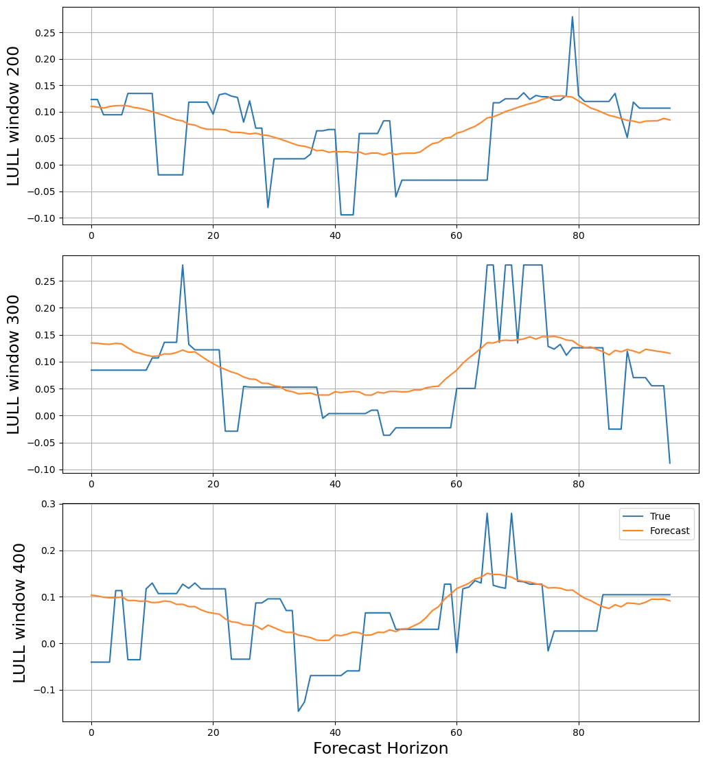
4. Evaluate Results

The AutoNHITS class contains a results tune attribute that stores information of each configuration explored. It contains the validation loss and best validation hyperparameter.

nf.models[0].results.get_best_result().config

{'learning_rate': 0.001,
 'max_steps': 1000,
 'input_size': 480,
 'batch_size': 7,
 'windows_batch_size': 256,
 'n_pool_kernel_size': [2, 2, 2],
 'n_freq_downsample': [24, 12, 1],
 'activation': 'ReLU',
 'n_blocks': [1, 1, 1],
 'mlp_units': [[512, 512], [512, 512], [512, 512]],
 'interpolation_mode': 'linear',
 'val_check_steps': 100,
 'random_seed': 8,
 'h': 96,
 'loss': MAE(),
 'valid_loss': MAE()}

from utilsforecast.plotting import plot_series                                                                                      
                                                                                                                                  
series = ['HUFL','HULL','LUFL','LULL','MUFL','MULL','OT']
series_id = series[3]  # 'LULL'

series_cutoffs = Y_hat_df.loc[Y_hat_df['unique_id'] == "LULL", 'cutoff'].unique()                                                
                                                        
for w_idx in [200, 300, 400]:
    cutoff = series_cutoffs[w_idx]
    plot_df = Y_hat_df.loc[Y_hat_df['cutoff'] == cutoff, ['unique_id', 'ds', 'y', 'AutoNHITS']]

    fig = plot_series(
        df=plot_df[['unique_id', 'ds', 'y']],
        forecasts_df=plot_df[['unique_id', 'ds', 'AutoNHITS']],
        ids=[series_id],
        models=['AutoNHITS'],
        max_insample_length=96
    )
    display(fig)

Finally, we compute the test errors for the two metrics of interest:

$\qquad MAE = \frac{1}{Windows * Horizon} \sum_{\tau} |y_{\tau} - \hat{y}_{\tau}| \qquad$ and $\qquad MSE = \frac{1}{Windows * Horizon} \sum_{\tau} (y_{\tau} - \hat{y}_{\tau})^{2} \qquad$

from utilsforecast.evaluation import evaluate
from utilsforecast.losses import mae, mse

eval_df = evaluate(
    df=Y_hat_df.drop(columns=["cutoff"]),
    metrics=[mae, mse],
    agg_fn="mean"
)

print('MAE: ', eval_df.iloc[0]["AutoNHITS"])
print('MSE: ', eval_df.iloc[1]["AutoNHITS"])

MAE:  0.24862242128243706
MSE:  0.17257850996828134

For reference we can check the performance when compared to previous ‘state-of-the-art’ long-horizon Transformer-based forecasting methods from the NHITS paper. To recover or improve the paper results try setting hyperopt_max_evals=30 in Hyperparameter Tuning.

Mean Absolute Error (MAE):

Horizon	NHITS	AutoFormer	InFormer	ARIMA
96	0.249	0.339	0.453	0.301
192	0.305	0.340	0.563	0.345
336	0.346	0.372	0.887	0.386
720	0.426	0.419	1.388	0.445

Mean Squared Error (MSE):

Horizon	NHITS	AutoFormer	InFormer	ARIMA
96	0.173	0.255	0.365	0.225
192	0.245	0.281	0.533	0.298
336	0.295	0.339	1.363	0.370
720	0.401	0.422	3.379	0.478

References

Cristian Challu, Kin G. Olivares, Boris N. Oreshkin, Federico Garza, Max Mergenthaler-Canseco, Artur Dubrawski (2021). NHITS: Neural Hierarchical Interpolation for Time Series Forecasting. Accepted at AAAI 2023.